With growing volumes of data, it becomes increasingly difficult for organizations to understand why their data changes. Organizations struggle to identify the root cause of critical trends and fluctuations, hindering their ability to make informed decisions. For example, a company might be left wondering, “What factors drove revenue growth between Q1 and Q2?” or “Why did the click-through rate on an advertisement decrease 5% over the last week?”
This kind of analysis requires tooling to inspect segments of the data at a time to find statistically significant key drivers. To help organizations perform this analysis interactively, and at scale, we are announcing the public preview of contribution analysis in BigQuery ML to help customers find insights and patterns in their data.
Contribution analysis allows you to analyze metrics of interest from your dataset across defined test and control subsets. It works by identifying combinations of ‘contributors’ that cause unanticipated changes, and it scales effectively by using pruning optimization to reduce the search space. This type of analysis can be used across several industries and use cases. Some examples include:
Telemetry monitoring: Analyze changes in logged events from software applications
Sales and advertisement: Explore user engagement for campaign and advertisement modifications based on click-through rates
Retail: Evaluate the impacts of pricing changes and inventory management practices to optimize stock levels
Healthcare: Investigate key factors impacting patient health to help tailor treatment plans and refine prognoses
How does it work?
To create a contribution analysis model in BigQuery ML, you provide the model with a single table that contains rows of both a control set of baseline data and a test set to compare against the control, a metric to analyze (e.g. revenue), and a list of contributors (e.g. product_sku, category, etc.). The model then identifies important slices of data identified by a given combination of contributor values, which we refer to as segments.
There are two different types of metrics you can analyze with contribution analysis: summable metrics and summable ratio metrics. Summable metrics summarize each segment of the data by aggregating a single measure of interest, such as revenue. Summable ratio metrics analyze the ratio between two measures of interest, such as earnings per share.
Contribution analysis models also offer pruning optimizations by default so you can get to insights faster through the Apriori pruning algorithm. Given a minimum support value, the model can prune the search space and quickly find relevant segments. The support value measures a segment’s size relative to the rest of the population. Pruning segments with low support values allows you to focus on the largest segments, while decreasing the query execution time.
A step-by-step example
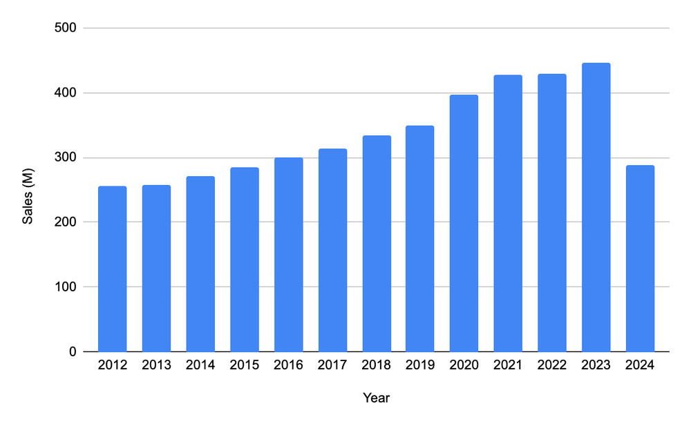
Let’s find key contributors of liquor sales with a summable contribution analysis model. In this example, we create a contribution analysis model to find key contributors that lead to changes in the ‘total_sales‘ metric between 2020 and 2021 in the Iowa liquor sales public dataset in BigQuery:
Step 1. Create the input dataset
Contribution analysis models take a single table as input. First, create a new table with the both the control data from 2020 and the test data from 2021, with the following columns:
store_name: Name of the store that ordered the liquor
city: City where the store that ordered the liquor is located
vendor_name: The vendor name of the company for the brand of liquor ordered
category_name: Category of the liquor ordered
item_description: Description of the individual liquor product ordered
total_sales: Total cost of the liquor ordered
is_test: Whether the order is a part of the 2020 control data (false), or the 2021 test data (true)
For a summable contribution analysis model, the following columns are required: a numerical metric column (total_sales in this example), a boolean column to indicate whether a record is in the test or control set, and one or more categorical columns which form the ‘contributors’.
<ListValue: [StructValue([(‘code’, ‘CREATE OR REPLACE TABLE bqml_tutorial.iowa_liquor_sales_control_and_test AS rn(SELECTrn store_name,rn city,rn vendor_name,rn category_name,rn item_description,rn SUM(sale_dollars) AS total_sales,rn FALSE AS is_testrnFROM `bigquery-public-data.iowa_liquor_sales.sales`rnWHERE EXTRACT(YEAR FROM date) = 2020rnGROUP BY store_name, city, vendor_name, rn category_name, item_description, is_testrn)rnUNION ALLrn(SELECTrn store_name,rn city,rn vendor_name,rn category_name,rn item_description,rn SUM(sale_dollars) AS total_sales,rn TRUE AS is_testrnFROM `bigquery-public-data.iowa_liquor_sales.sales`rnWHERE EXTRACT(YEAR FROM date) = 2021rnGROUP BY store_name, city, vendor_name, rn category_name, item_description, is_testrn);’), (‘language’, ”), (‘caption’, <wagtail.rich_text.RichText object at 0x3e3bf2b1f550>)])]>
The output table has 901,859 rows.
Step 2. Create the model
To create a contribution analysis model, you can use the CREATE MODEL statement. In this example, we are interested in the total_sales summable metric and in the store_name, city, vendor_name, category_name, and item_description as potential contributor dimensions. To reduce model creation time and exclude small segments of data, we are adding a minimum support value of 0.05. The minimum support value of 0.05 guarantees that output segments must make up at least 5% of the total_sales in the underlying test or control data.
It takes around one minute to create the model.
<ListValue: [StructValue([(‘code’, “CREATE OR REPLACE MODEL bqml_tutorial.iowa_liquor_sales_contribution_analysis_modelrn OPTIONS(rn model_type = ‘CONTRIBUTION_ANALYSIS’,rn contribution_metric = rn ‘sum(total_sales)’,rn dimension_id_cols = [‘store_name’, ‘city’,rn ‘vendor_name’, ‘category_name’, ‘item_description’],rn is_test_col = ‘is_test’,rn min_apriori_support = 0.05rn) ASrnSELECT * FROM bqml_tutorial.iowa_liquor_sales_control_and_test;”), (‘language’, ”), (‘caption’, <wagtail.rich_text.RichText object at 0x3e3bf2b1f0a0>)])]>
Step 3. Get insights from the model
With the model created in Step 2, you can use the new ML.GET_INSIGHTS function to retrieve the insights from the sales data.
<ListValue: [StructValue([(‘code’, ‘SELECT rn contributors,rn metric_test,rn metric_control,rn difference,rn relative_difference,rn unexpected_difference,rn relative_unexpected_difference,rn apriori_supportrn FROM ML.GET_INSIGHTS(rn MODEL bqml_tutorial.iowa_liquor_sales_contribution_analysis_model)rnORDER BY unexpected_difference DESC;’), (‘language’, ”), (‘caption’, <wagtail.rich_text.RichText object at 0x3e3bf2b1fd00>)])]>
The output has been sorted by the unexpected difference, which measures how much the segment’s test value differs from the expected value of the segment.
The expected value of a segment depends on the existing relationship between the test and control across the whole population, excluding the segment in question. To calculate the expected value of a segment, we first compute the ratio across the aggregate metric_test and aggregate metric_control for the rest of the population. By multiplying this ratio by the target segment’s metric_control, we’re able to find the expected test value. Then, we calculate the unexpected difference as the difference between the segment’s test value and the expected test value. For more information on all of the output metric calculations, see ML.GET_INSIGHTS function.
From the insights generated by ML.GET_INSIGHTS, we can see how different combinations of contributors led to an unanticipated increase in total liquor sales. For example, the `100% AGAVE TEQUILA` category (row 3) drove an additional $6,662,926 in total sales from 2020 to 2021, with $5,528,662 of that growth considered unexpected, indicating that this segment is outperforming the population as a whole. From the `relative_unexpected_difference` metric, we can see this segment grew an additional 30% more than expected. Since we configured the model to prune segments with less than 5% of support in the data, we know this is a significantly large segment of the data.
Take the next step
Contribution Analysis is now available in BigQuery in preview. For more details, please see the tutorial and the documentation.