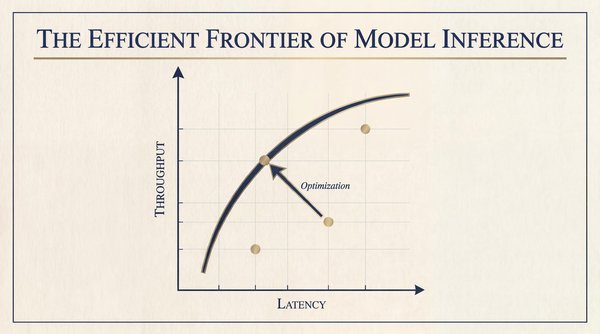
Every dollar that you spend on model inference buys you a position on a graph of latency and throughput. On this plot is a curve of optimal configurations, where you’ve squeezed the maximum possible performance from your hardware. That curve, borrowed from portfolio theory in finance, is the efficient frontier.
With the assumption that you have a fixed budget for hardware, you can trade latency for throughput. But, you can’t improve one aspect without sacrificing the other, unless the frontier curve itself moves. There are two fundamentally different dynamics at play, and this is the central insight for anyone running LLMs in production.
The first dynamic is getting to the frontier, which involves applying the full stack of techniques available to you today. This part is within your control. Continuous batching, paged attention, intelligent routing, speculative decoding, and quantization all exist right now. If you’re not using these techniques, you’re operating below the frontier and leaving performance on the table.
The second dynamic is that the frontier itself is constantly moving outward. This part is largely outside of your control. Researchers publish new algorithms. Hardware vendors ship new architectures. Open-source projects mature. Each breakthrough redefines what’s physically achievable and expands the curve so that yesterday’s optimal configuration is today’s inefficiency.
Your job as a platform engineer is to stay as close to the frontier as possible as you build infrastructure that’s flexible enough to absorb each new advance as it arrives. This article gives you the tools to do just that.
Why inference has an efficient frontier
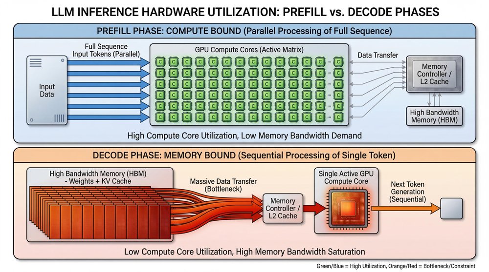
Every LLM request has two computational phases, and they can have bottlenecks for different hardware resources.
1. Prefill (Compute-Bound): In this phase, the GPU processes your entire input prompt at one time to build the key-value (KV) cache for the attention mechanism. Because the instructions are batch-processed in parallel, the GPU’s compute cores (tensor cores) are highly utilized. This phase is fast and efficient: the processors have all of the data that they need, immediately available, to perform massive matrix multiplications. Longer prompts just mean more computations.
2. Decode (Memory-Bandwidth-Bound): This phase generates new tokens, one at a time, autoregressively. To generate only one single token, the GPU can’t batch the work. It must fetch the entire model’s weights and the growing KV cache from High-Bandwidth Memory (HBM) into the compute cores. Then, the GPU needs to calculate that one token, and then waits to do it all over again for the next one.
This mismatch is the fundamental reason that the frontier exists. You can’t optimize a single system for both phases simultaneously without making some tradeoffs.
The two axes of inference
Instead of risk and return, the efficient frontier of LLM inference measures a different fundamental tradeoff, with the assumption that the hardware budget is fixed:
| Axis | Key metrics measured | Hardware constraint |
| Latency (the X-Axis) | Time to First Token (TTFT) + Time Between Tokens (TBT) | Compute (prefill) and memory bandwidth (decode) |
| Throughput (the Y-Axis) | Total tokens per second across all concurrent users | Batch size × memory capacity |
Cost is the constraint that buys the graph of latency and throughput itself. If you increase your hardware budget, or the industry invents a new algorithmic breakthrough, the entire frontier curve shifts outward. For a given budget and software stack, you can apply today’s best practices to move from a sub-optimal point towards that frontier.
Getting to the frontier: Five techniques within your control
Most production inference systems today operate below the frontier. They’re leaving performance on the table, not because better techniques don’t exist, but because they haven’t adopted them yet. Everything described in this section is available today. If you’re not applying these techniques, you’re choosing to operate below the curve.
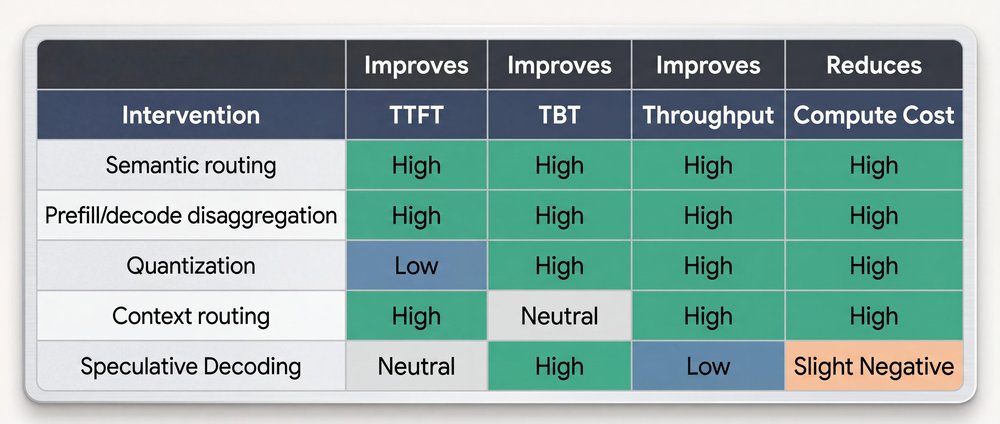
1. Semantic routing across model tiers
Not every query needs a 400B parameter model. Simple classification, summarization, or formatting tasks can be routed to smaller, quantized models that are orders of magnitude cheaper per token. A lightweight classifier at the gateway edge analyzes query complexity and routes accordingly: frontier-class models for hard reasoning, and small models for everything else.
Semantic routing pushes your system dramatically closer to its theoretical maximum throughput, and avoids wasted cycles on easy tasks, without sacrificing aggregate output quality.
2. Prefill and decode disaggregation
Physically separating prefill and decode phases onto different hardware is one of the most architecturally significant optimizations available today.
The prefill phase needs compute-dense GPUs. The decode phase needs high-bandwidth memory. If you force both phases onto the same GPU, then one resource is always underutilized.
To push both phases toward their theoretical hardware limits independently, run dedicated prefill clusters and decode clusters. Connect these clusters with high-speed networks that transfer only the compressed KV cache state to the same GPU, then one resource is always underutilized.
3. Quantization: Trading precision for speed
When you reduce model weights from FP16 to the INT8 or INT4 formats, you can reduce the memory footprint to half or a quarter. Because the decode phase is memory-bandwidth-bound, 4-bit weights can be read up to 4× faster than 16-bit weights. This approach provides a direct TBT improvement.
The tradeoff is quality because naive quantization degrades model outputs. Modern techniques like Activation-aware Weight Quantization (AWQ) and GPTQ preserve the quality of sensitive weights, but aggressively compress others, to achieve near-FP16 quality at INT4 speeds.
4. Context routing: The biggest lever that most teams miss
In a production deployment with dozens of model replicas, the routing layer is where the biggest competitive advantages are won or lost today.
In 2026, prefix caching is foundational. If ten users ask questions about the exact same 100-page RAG document, or use the identical massive system prompt, you shouldn’t run the compute-heavy prefill phase ten times. You should compute the KV cache once, store it, and then let the other nine users reuse it. This approach slashes TTFT by up to 85% and drastically reduces compute costs.
But, there’s a catch: a standard L4 load balancer scatters requests randomly. If user 2’s request lands on a different GPU than user 1’s request, the prefix cache is useless. The system has to recompute the cache from scratch.
This is why context-aware L7 routing is the differentiator. An intelligent router inspects the incoming prompt’s prefix and intentionally routes the request to the specific pod that already holds that context in its cache. You stop wasting compute power on redundant work and instantly push your latency and throughput closer to the physical limits of your hardware.

5. Speculative decoding
Remember: during the decode phase, tensor cores are mostly idle because there’s a bottleneck on memory bandwidth. Speculative decoding exploits this wasted computation power.
A small, fast “draft” model generates several candidate tokens cheaply. The large target model then verifies all of the candidates in a single forward pass, which is a parallel compute-bound operation, rather than a sequential memory-bound one. If the draft model predicted the candidates correctly, you’ve generated 4-5 tokens for the memory cost of one.
This approach directly breaks the TBT floor set by memory bandwidth. If you’re not using speculative decoding for latency-sensitive workloads, you’re not leveraging one of the most impactful optimizations available.
Although the addition of a draft model can introduce some operational complexity and slightly increase compute costs, the draft model is relatively tiny compared to the main model. This tradeoff for latency is worthwhile.
Note that some newer models have introduced self-speculative decoding, which eliminates the overhead of managing a second model. These models use specialized internal layers (often called prediction heads) that are trained to predict extra future tokens simultaneously. These models generally achieve a highly meaningful token hit rate.
Case study: How Vertex AI moved closer to the frontier
The Vertex AI engineering team moved closer to the frontier when they adopted GKE Inference Gateway, which is built on the standard Kubernetes Gateway API. Inference Gateway intercepted requests at Layer 7 and added two critical layers of intelligence:
-
Load-aware routing: It scraped real-time metrics (like KV cache utilization and queue depth) directly from the model server’s Prometheus endpoints. This process routes requests to the pod that can serve them the fastest.
-
Content-aware routing: Crucially, it inspected request prefixes and routed traffic to the pod that already held that specific context in its KV cache. This process avoids expensive re-computation.
When the production workloads were migrated to this intelligent routing architecture, the Vertex AI team proved that optimizing the network layer is key to unlocking performance at scale. Validated on production traffic, the results were stark:
-
35% faster TTFT for Qwen3-Coder (context-heavy coding agent workloads)
-
2x better P95 tail latency (52% improvement) for DeepSeek V3.1 (bursty chat workloads)
-
Doubled prefix cache hit rate (optimized from 35% to 70%)
The bottom line
LLM inference has an efficient frontier, which represents a hard boundary where latency and throughput are optimally balanced for a given compute budget.
Getting to that frontier is within your control. The techniques exist today: continuous batching, paged attention, intelligent L7 routing, speculative decoding, quantization, and prefill and decode disaggregation. The GKE Inference Gateway case study shows that routing alone, without changing hardware, models, or cluster size, cut TTFT by 35% and doubled cache efficiency. If you’re not applying the full stack, you’re operating below the curve and overpaying for every token.
The frontier itself keeps moving outward. This part is outside of your control. Researchers publish new algorithms, hardware vendors ship new architectures, and open-source serving frameworks integrate these algorithms and architectures. Something that was cutting-edge optimization 18 months ago became a baseline table stake. Your job isn’t to predict which breakthrough comes next; it’s to build infrastructure flexible enough to absorb it when it arrives.
The organizations that will win on inference economics aren’t the ones with the most GPUs. They’re the ones that systematically close the gap to today’s frontier while they stay ready for tomorrow’s.
Have you applied any of these optimization techniques to your own LLM inference workloads? I’d love to hear about your experience! Share what you’ve built with me on LinkedIn, X, or Bluesky!